VLOOKUP and ARRAYFORMULA are powerful tools in Google Sheets that work together to search for specific data within a large dataset. VLOOKUP retrieves the desired information from a table, while ARRAYFORMULA allows you to apply this formula across multiple rows or columns simultaneously.
VLOOKUP helps find specific values in a table, and with ARRAYFORMULA, you can apply this operation to multiple rows at once in Google Sheets.
The VLOOKUP function in Google Sheets or Excel is used to search for a value in the first column of a range (or table) and return a value in the same row from another column. It stands for Vertical Lookup.
Syntax
VLOOKUP( search_key, range, index, [ is_sorted ] )
- search_key: The value you want to look for in the first column of the range.
- range: The range of cells to search in. The first column is where the search is performed.
- index: The column number (relative to the range) from which to return the value.
- is_sorted (optional):

How to use VLOOKUP to retrieve data based on a unique key (e.g., Stock ID)
First select that cell where you want to enter the formula and type the equals sign (=) and then type VLOOKUP and press Tab on your keyboard. Now you need to add the values you want to lookup into your formula.
Formula:=VLOOKUP( A15 , $A$3:$F$10, 2, 0 )
Result:
Looks for the value 452 (Stock ID) in the first column of range $A$3:$F$10"ASICS" retrieved as results.
Explanation of Key Components
search_key(A15):contains the Stock ID (452).range($A$3:$F$10):Make the range absolute, meaning it doesn’t change when formulas are dragged across or copied to other cells.index (2):The column index (1, 2, 3, 4, etc.) determines which column’s data is returned. Here,2retrieves data from the second column (Brand Name).is_sorted (Last argument ensure an exact match for the0orFALSE):search_key. If not found, will return an error(#N/A).- The result corresponds to the Stock ID provided in
A15(452).

The VLOOKUP function in Google Sheets is an essential tool for retrieving specific information, such as Brand Names, Product Types, Purpose, Cost Price, or Sell Price, using a unique key like a Stock ID. It works by searching for the search_key in the first column of a defined range and returning data from a specified column based on the index.
To ensure accurate results, the range should be absolute ($A$3:$F$10), and the is_sorted argument should be set to 0 for an exact match or TURE for approximate match, when TRUE, the first column must be sorted in ascending order. With this setup, VLOOKUP simplifies the process of extracting organized data from tables, making it ideal for managing and analyzing structured datasets
Array compatibility with VLOOKUP
Array compatibility in VLOOKUP allows you to perform multiple lookups simultaneously. Here are the key aspects:
Combining VLOOKUP and ARRAYFORMULA enables you to efficiently search for and retrieve data in bulk from a large dataset in Google Sheets.
Above we use the single Value Lookup =VLOOKUP(A3, $B$3:$D$10, 2, FALSE)

Array Lookup (Multiple Values) =VLOOKUP(A3:A10, $B$3:$D$10, 2, FALSE)
In this scenario, instead of using a single Stock ID as the lookup value, multiple Stock IDs (A2:A10) are provided as an array. The VLOOKUP function searches for each Stock ID in the first column of the range $B$3:$D$10 and retrieves the corresponding values from the second column
Key Points:
- When you provide an array of search keys (like
A3:A10),VLOOKUPautomatically returns an array of results - The
ArrayFormulawill spill into adjacent cells in Google Sheets - Each value in your search array will be looked up independently
Common Array Use Cases:
- Looking up multiple product IDs at once
- Comparing two columns of data
- Creating summary tables from raw data
ArrayFormula with multiple index arguments

=ArrayFormula(VLOOKUP(A3:A10,$A$3:$F$10,{2,3,4,5},0))
This formula looks up the ProductID values in A3:A10 from the first column, then retrieves Brands Name (2nd column), Product Types (3rd column), Purpose (4th column) and Sell Price (5th column).
This way, you can compare multiple columns of products data across different stores efficiently.
Key Considerations for Array Formulas
- Array formulas can slow down performance with large datasets, requiring optimization to manage computational demands and improve efficiency.
- Array formulas need empty cells to spill results correctly. Lack of space causes errors, ensuring adjacent cells are clear.
- Column indexing in array formulas allows retrieval of multiple columns simultaneously, simplifying data extraction and reducing the need for multiple formulas.
If you have any questions, need assistance, or encounter challenges, feel free to share your concerns in the comments. The CountLen team is dedicated to providing quick and effective solutions. If you notice any inaccuracies or misleading information, please provide feedback—we’re here to support you!