If you want to create custom calendar in Google Sheets than you’re at right place, by creating a custom calendar its useful for specific projects or layouts. Hence, Google Sheets offers built-in calendar functionality but its work only where date formats placed in the cell there you need to double click on the date, a custom calendar pop-up appear, where you simply change the date or month by using that pop-up easily.
How to Generate a Custom Calendar Similar to Google Calendar in Google Sheets:

Creating a calendar in Google Sheets that mimics the default Google Calendar format is simple. In the above example, we aim to generate a calendar format similar to the default layout in Google Sheets. By entering the provided formula in cell C2 and pressing Enter, you can easily generate a monthly or yearly calendar. With a few adjustments, such as formatting text or adding borders, you’ll have a calendar closely resembling the one found in Google Sheets as defaults. Here we discus about two method for creating a custom calendar:
First, Using Combination of Three Functions:
SEQUENCEfunction:
SEQUENCE(rows, columns, start, step)DATEfunction:
DATE(year, month, day)WEEKDAYfunction:
WEEKDAY(date, [type])
In the first method choose a cell in your Google Sheet where you want the calendar to appear. The below image shown the formula placed in a specific cell and results come out.

Short formula, step to Generate a Calendar Using a Formula in Google Sheet:
- Insert the Formula: Use the following formula in the designated cell to generate the calendar grid:
=SEQUENCE(6,7,DATE($B$5,$B$6,1)- (WEEKDAY(DATE($B$5,$B$6,1))-1),1)
- Paste this formula into cell D4 (or any other starting cell as your desire)
- Check Year and Month Values: Ensure that cell B5 contains the year and cell B6 contains the month. If you’re using different cells for year and month, replace
$B$5 and $B$6in the formula with the appropriate cell references. - Setup Calendar Sheet: Here we take the sheet “Calendar”, set A5 (Year) to 2025 and A6 (Month) to 9, using dropdowns or manual entries.
- In row range D3:J3, manually enter the first letter of the days of the week (S,M,T,W,T,F,S).
- Result: After entering the formula in cell D4, press Enter, and the calendar will instantly appear in a 7×6 grid showing the correct dates for the specified month.
Second, Using Combination of Eight Functions:
The second Function is some large but result is more reliable and easily decorate the month chart on Google Sheets, which using the set of or combination of eight below formulas:
- ArrayFormula function:
ARRAYFORMULA(array_formula) - IF function:
IF(logical_expression, value_if_true, value_if_false) - MONTH function:
MONTH(date) - DATE function:
DATE(year, month, day) - YEAR function:
YEAR(date) - SEQUENCE function:
SEQUENCE(rows, columns, start, step), the function, which is use in our previous post,
Auto Fill Serial Numbers, Using Function in Google Sheets - WEEKDAY function:
WEEKDAY(date, [type]) - EOMONTH function:
EOMONTH(start_date, months)
You can use the other formula instead of the above describe (sort formula), if you desire auto fill the name of day (Sun, Mon, Tue, Wed, Thu, Fri and Sat) then use the below function:

={{"Sun","Mon","Tue","Wed","Thu","Fri","Sat"};ARRAYFORMULA(IF(MONTH(DATE(YEAR(B1), MONTH(B1),SEQUENCE(7,7,-1*(WEEKDAY(EOMONTH(B1,-1)+1)+5),1)))=MONTH(B1), SEQUENCE(7,7,-1*(WEEKDAY(EOMONTH(B1,-1)+1)+5),1),"⋅"))}
Let’s Break Down how it Works:
{{"Sun","Mon","Tue","Wed","Thu","Fri","Sat"};
This part creates a static array containing the names of the days of the week and auto-fill the first row of the calendar grid with these names, similar to how days appear in most calendars. If you want week days name in other formats, replace value accordingly.ARRAYFORMULA(….)
TheARRAYFORMULAfunction enables the application of the formula across an entire range of cells, allowing the rest of the formula to output multiple results in a grid format.DATE(YEAR(B1), MONTH(B1),SEQUENCE(….))
This part create a specific date based on the year and month from cellB1. TheYEAR(B1)andMONTH(B1)pull the year and month from the input in cellB1, whileSEQUENCE(….) is used to create a series of dates to fill the calendar grid.YEAR(B1): Extracts the year from the date inB1.MONTH(B1): Extracts the month from the date inB1.SEQUENCE(7,7,-1*(WEEKDAY(EOMONTH(B1,-1)+1)+5),1),"⋅")
This is the core logic that generates a 7×7 grid of numbers, each representing a day of the month, starting from the correct day of the week.IF(MONTH(DATE(....)=MONTH(B1), SEQUENCE(....), ".")
This part ensure that only the days of the current month are displayed in the gird and"."for dates that fall outside of the current month, this symbol( . )is displayed, visually separating days that do not match to the current month.
={{"Sun","Mon","Tue","Wed","Thu","Fri","Sat"};ARRAYFORMULA(IF(MONTH(DATE(YEAR(B1),MONTH(B1),SEQUENCE(7,7,-1*(WEEKDAY(EOMONTH(B1,-1)+1)+5),1)))=MONTH(B1),SEQUENCE(7,7,-1*(WEEKDAY(EOMONTH(B1,-1)+1)+5),1),"•"))}
Summary of How the Formula Works:
- The formula first fill the day names Sunday to Saturday (e.g.
"Sun","Mon","Tue","Wed","Thu","Fri","Sat") at the top or first row where the formula put in the cell. - Next it generates a 7×7 grid representing the days of the month, adjusting for the starting day and ensuring the days of the previous or next month are represented by
".". - By referencing
B1for the year and month, the calendar adapts dynamically to any input.
This setup makes it easy to generate a calendar automatically, along with correctly aligned weekday headers and blank spaces for days outside the cureent month.

Second method, using Apps Script:
This method involves writing a script to generate the calendar programmatically or you can simply copy and paste the below script.
function createCalendar() {
var sheet = SpreadsheetApp.getActiveSheet();
var dateCell = sheet.getRange("A1");
var dateValue = dateCell.getValue();
if (!(dateValue instanceof Date)) {
Browser.msgBox("Please check if a valid date in cell A1 or not.");
return;
}
var date = new Date(dateValue);
var year = date.getFullYear();
var month = date.getMonth();
var firstDay = new Date(year, month, 1);
var lastDay = new Date(year, month + 1, 0);
// If you have alread content in the sheets getRange than Clear existing content
sheet.getRange(1, 1, 8, 7).clearContent();
// Set month and year
sheet.getRange(1, 1).setValue(Utilities.formatDate(date, Session.getScriptTimeZone(), "MMMM yyyy"));
// Set headers ("If you want to change the format days name than you customise accordingly")
var days = ["Sun", "Mon", "Tue", "Wed", "Thu", "Fri", "Sat"];
sheet.getRange(2, 1, 1, 7).setValues([days]);
var day = 1;
var startRow = 3; // Start filling dates from the third row
for (var i = 0; i < 6; i++) { // Up to 6 weeks
var row = [];
for (var j = 0; j < 7; j++) {
if ((i === 0 && j < firstDay.getDay()) || day > lastDay.getDate()) {
row.push("");
} else {
row.push(day);
day++;
}
}
sheet.getRange(startRow + i, 1, 1, 7).setValues([row]);
if (day > lastDay.getDate()) break;
}
// Auto-resize columns
sheet.autoResizeColumns(1, 7);
}
What is the parameter in the context (javascript) – sheet.getRange(2, 1, 1, 7):
sheet.getRange(startRow, startColumn, numRows, numColumns)2: This is thestartRow.It means the range starts from the 2nd row of the sheet.1: This is thestartColumn.It means the range starts from the 1st column (column A) of the sheet.1: This isnumRows.It specifies that the range should include only 1 row.7: This isnumColumns.It specifies that the range should include 7 columns.
So, sheet.getRange(2, 1, 1, 7) selects a range that:
- Starts at cell A2 (2nd row, 1st column)
- Spans 1 row down
- Spans 7 columns across (from A to G)
This effectively selects the range A2:G2 in the sheet.
How to Use Apps Script, Follow the instruction as given below:

Apps Script, Step wise how to generate the calendar:

Follow the steps:
- Go to the Extensions Tab in Google Sheets
- Tap on the Apps Script in drop down list
- Type or paste the above script in editor(side strips) file Code.gs and save
- Click on the Run Button in control toolbar
- Review permission
- Choose an account
- Allow access
- If show warning go to calendar (unsafe)
- Again click on the Run Button, if show execution started and completed, go to the Google Sheets and check the result as shown left.
So, if you want to create your own costume calendar by month, simply way to create that project for your purpose. You can use the both way to generate the calendar first by formula enter in specify cell or using the apps script belong to the calendar creation.


