Mastering Age Calculation in Google Sheets: A Practical Guide
If you’ve ever struggled with converting a date of birth (DOB) into age, don’t worry—you’re in the right place! This guide will walk you through different methods to calculate age in years, months, or even days using built-in Google Sheets functions.
Google Sheets offers several built-in functions to calculate age efficiently. This guide will explore different methods, including the DATEDIF function, which provides a straightforward way to measure the difference between two dates, and the YEARFRAC function, which returns age in a decimal format.
Understanding How Dates Work in Google Sheets
Before calculating age in Google Sheets, it’s essential to understand how dates work. Unlike regular text, dates in Google Sheets are stored as numeric serial values. Each date corresponds to a specific number, with January 1, 1900, assigned the value 1, and each following day increasing by 1. This system allows for easy date calculations, such as finding differences between dates or adding days, months, or years.
Among the most effective formulas are DATEDIF, which quickly finds the difference between two dates, and YEARFRAC, which provides age in a decimal format. With these functions, you’ll be able to calculate ages with precision, improving accuracy in reports and records.
Here are several functions or methods to calculate the difference between two dates in terms of years, months, and days.
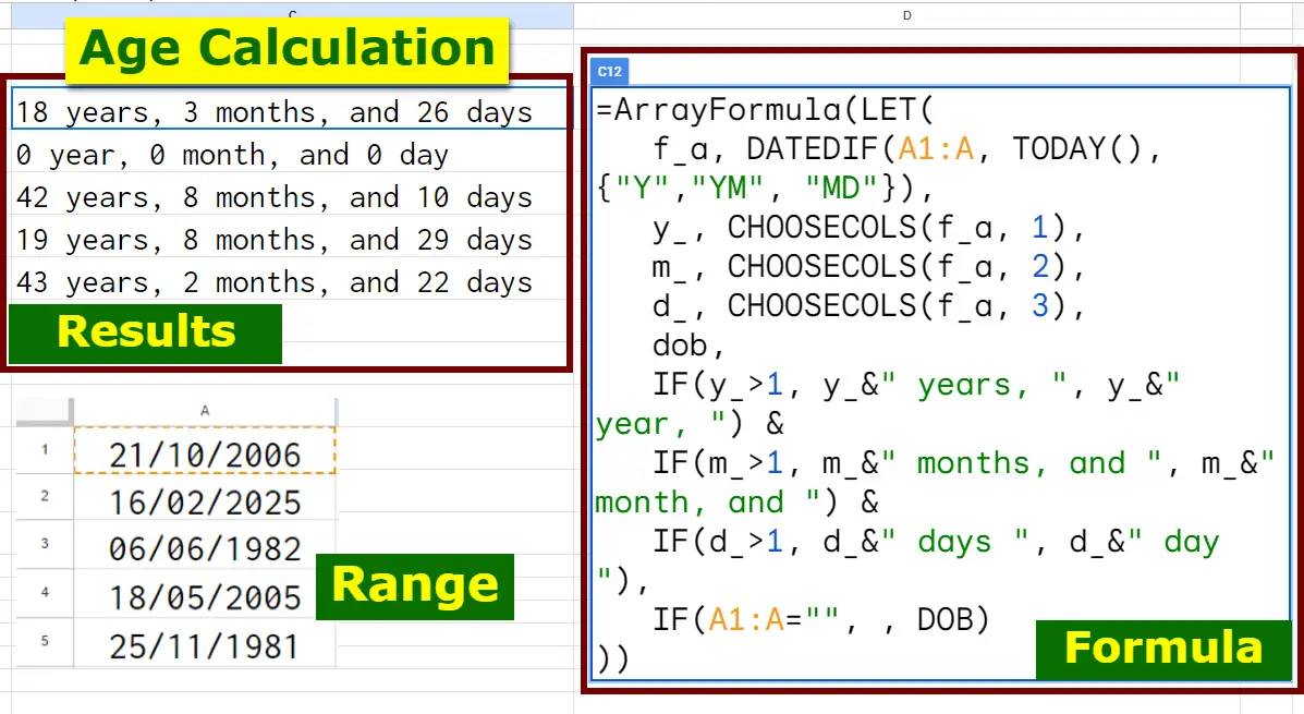
1. Understanding an ArrayFormula to Calculate the Age in Google Sheets
=ArrayFormula(LET(
f_a, DATEDIF(A1:A, TODAY(), {"Y","YM", "MD"}),
y_, CHOOSECOLS(f_a, 1),
m_, CHOOSECOLS(f_a, 2),
d_, CHOOSECOLS(f_a, 3),
dob,
IF(A1:A=TODAY(), "Today",
IF(y_>1, y_&" years, ", y_&" year, ") &
IF(m_>1, m_&" months, and ", m_&" month, and ") &
IF(d_>1, d_&" days ", d_&" day ")
),
IF(A1:A="", , DOB)
))
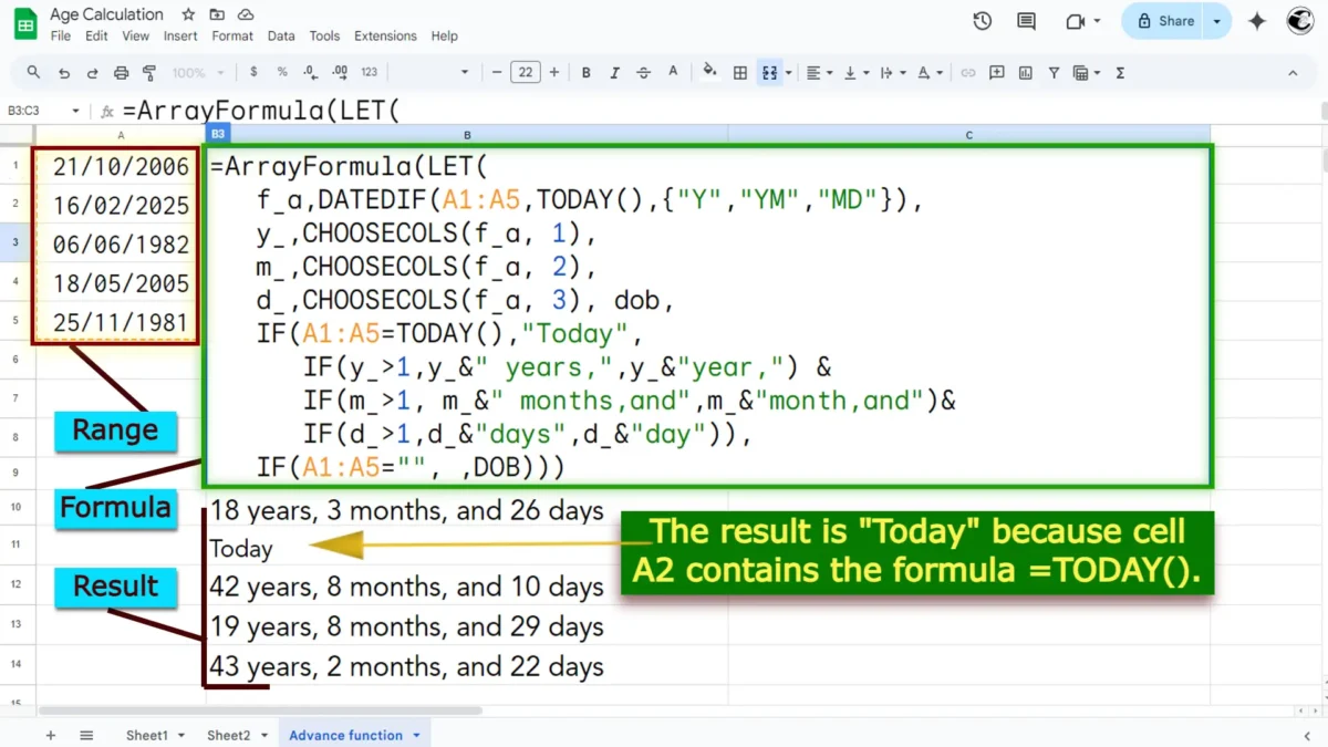
An ArrayFormula that calculates age in years, months, and days for a list of birthdates (A1:A). It formats the result into a readable string like:
18 years, 3 months, and 26 days
OR
=LET(
f_a, ArrayFormula(DATEDIF(A1, TODAY(), {"Y","YM", "MD"})),
y_, CHOOSECOLS(f_a, 1),
m_, CHOOSECOLS(f_a, 2),
d_, CHOOSECOLS(f_a, 3),
IF(y_>1, y_&" years, ", y_&" year, ") &
IF(m_>1, m_&" months, and ", m_&" month, and ") &
IF(d_>1, d_&" days ", d_&" day ")
)
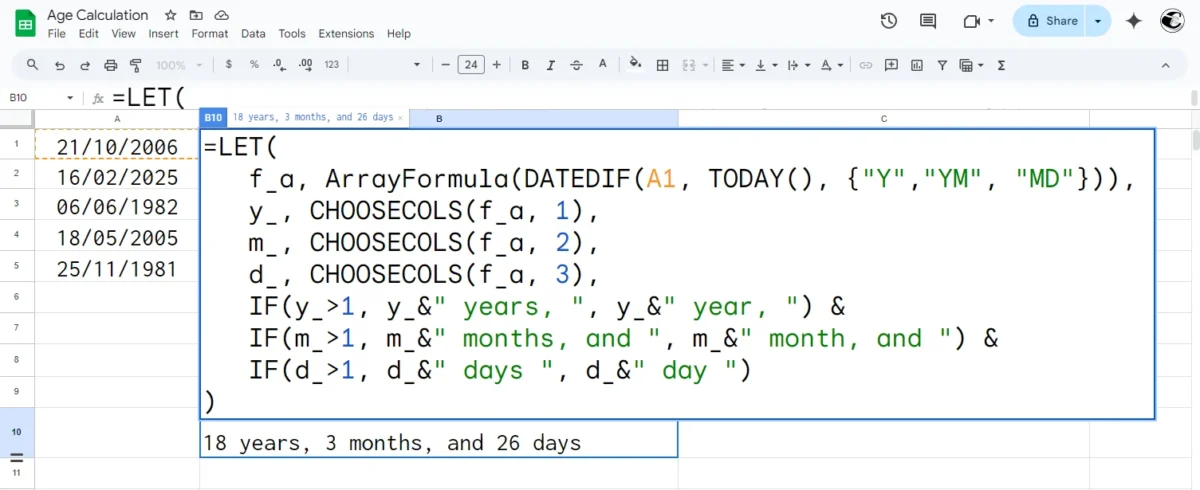
OR
=ArrayFormula(LET(
f_a, DATEDIF(A1:A, TODAY(), {"Y","YM", "MD"}),
y_, CHOOSECOLS(f_a, 1),
m_, CHOOSECOLS(f_a, 2),
d_, CHOOSECOLS(f_a, 3),
dob,
IF(y_>1, y_&" years, ", y_&" year, ") &
IF(m_>1, m_&" months, and ", m_&" month, and ") &
IF(d_>1, d_&" days ", d_&" day "),
IF(A1:A="", , DOB)
))
2. Using DATEDIF Function (Years, Months, and Days)
The DATEDIF function calculates the difference between two dates in different units.
Formula:=DATEDIF(A1,TODAY(),"Y")&" Years, "&DATEDIF(A1,TODAY(),"YM")&" Months, "&DATEDIF(A1,TODAY(),"MD")&" Days"

Explanation:
DATEDIF(A1,TODAY(),"Y")→ Gets the total number of full years
2025 – 2006 = 18 yearsDATEDIF(A1,TODAY(),"YM")→ Gets the remaining months after full years
From October 2024 to February 2025 = 3 monthsDATEDIF(A1,TODAY(),"MD")→ Gets the remaining days after full months
From 21st to 16th = -5 days (adjustment needed, so subtract one month and add days from previous month)
Example and Output:
Adjusted Months: 3 → 2 months
Adjusted Days: (31-21) + 16 = 26 days
If A1 = 21-October-2006 and today is 16-Feb-2025, the output will be:
“18 Years, 3 Months, 26 Days”
3. Using DATEDIF with Weeks Instead of Days
To display the remaining time in weeks instead of days, divide the days by 7.
=DATEDIF(A1,TODAY(),"Y")&" Years, "&DATEDIF(A1,TODAY(),"YM")&" Months, "&ROUND(DATEDIF(A1,TODAY(),"MD")/7)&" Weeks"
Explanation:
ROUND(DATEDIF(A1,TODAY(),”MD”)/7) → Converts remaining days into weeks.
Example and Output:
Convert Days to Weeks: 26 / 7 = 3.71 ≈ 4 weeks
If A1 = 21-October-2006 and today is 16-Feb-2025, the output might be:
“18 Years, 3 Months, 4 Weeks”
4. Using INT for More Precise Year, Month & Day Calculation
This method avoids potential DATEDIF errors in some cases.
Formula:=INT(YEARFRAC(A1,TODAY())) & " Years, " & INT((YEARFRAC(A1,TODAY())-INT(YEARFRAC(A1,TODAY())))12) & " Months, " & ROUND((TODAY()-EDATE(A1,12INT(YEARFRAC(A1,TODAY()))+INT((YEARFRAC(A1,TODAY())-INT(YEARFRAC(A1,TODAY())))*12)))/7,0) & " Weeks"

Explanation:YEARFRAC(A1,TODAY()) → Calculates fractional years.INT(… * 12) → Extracts remaining months.INT(… / 7) → Converts remaining days into weeks.
Example and Output:
“18 Years, 3 Months, 4 Weeks”
5. If You Need Age in Just Total Weeks
If you need only the total age in weeks, use:
Formula:=INT((TODAY()-A1)/7) & " Weeks"
Explanation:(TODAY()-A1)/7 → Finds total weeks.INT(…) → Converts it to a whole number.
Example Output:
“956 Weeks”
6. Using MOD for More Accurate Age Calculation
A more precise formula using MOD() to handle months and weeks correctly.
Formula:=DATEDIF(A1,TODAY(),"Y")&" Years, "&MOD(DATEDIF(A1,TODAY(),"M"),12)&" Months, "&INT(MOD(DATEDIF(A1,TODAY(),"D"),30.4375)/7)&" Weeks"

Explanation:MOD(DATEDIF(A1,TODAY(),"M"),12) → Gets only the remaining months.MOD(DATEDIF(A1,TODAY(),"D"),30.4375)/7 → Converts leftover days into weeks.
Example Output:
“18 Years, 3 Months, 4 Weeks”
The value 30.4375 in the formula represents the average number of days in a month over a year.
A year has 365.25 days on average (including leap years), and since a year has 12 months, the average number of days per month is:
365.25/12 = 30.4375
- Months have different lengths (28 to 31 days).
- Using 30.4375 provides a more accurate calculation over a long period.
7. If You Need Age in Just Total Days
Where A1 = 21-October-2006 and TODAY() = 16-FEBRUARY-2025
| Year | Days Count |
|---|---|
| 2006 (Oct 21 – Dec 31) | 72 days |
| 2007-2023 (17 years) | (17 × 365) + 5 leap days = 6209 days |
| 2024 (Jan 1 – Dec 31, Leap Year) | 366 days |
| 2025 (Jan 1 – Feb 16) | 47 days |
| Total Days | 72 + 6209 + 366 + 47 = 6693 days |
To get total age in days, use:
Formula:=TODAY()-A1 & " Days"
Example Output:
“6693 Days”
8. YEARFRAC Function in Google Sheets
The YEARFRAC function in Google Sheets calculates the fractional difference between two dates in years. It provides age in decimal format, which is useful when you need more precision beyond whole years.
Syntax:YEARFRAC(start_date, end_date, [basis])
start_date– The beginning date (e.g., birthdate).end_date– The ending date (e.g., today’s date or a reference date).basis– Determines how the function counts days in a year. Default is 0 (360-day year).

Example Usage:
Calculate Age in Decimal Years=YEARFRAC(A1, TODAY())
If A1 = 21-Oct-2006, and today is 16-Feb-2025, the result would be 18.32328767 (approx.)
Using a Specific Date Instead of TODAY=YEARFRAC(A1, DATE(2025,12,31))
This calculates the age on December 31, 2025.
Rounding to Whole Years
To get only the whole number of years:=INT(YEARFRAC(A1, TODAY()))
This removes the decimal portion, giving only 18 years.
Understanding the Optional “Basis” Argument:
=YEARFRAC(A1, TODAY(), 1)This considers leap years and provides a more precise age.
| Basis | Description |
|---|---|
| 0 (default) | 360-day year (US NASD method) |
| 1 | Actual days in a year (365 or 366 for leap years) |
| 2 | 360-day year (European method) |
| 3 | 365-day year (ignores leap years) |
| 4 | 360-day year (standard) |
Summary of All Methods:
- Where A1=21-October-2006
TODAY()=16-FEBRUARY-2025
| Method | Formula | Example Output |
|---|---|---|
| Years, Months, Days | =DATEDIF(A1,TODAY(),"Y")&" Years, "& | 18 Years, 3 Months, 26 Days |
| Years, Months, Weeks | =DATEDIF(A1,TODAY(),"Y")&" Years, "& | 18 Years, 3 Months, 4 Weeks |
| INT Method | =INT(YEARFRAC(A1,TODAY())) & " Years, " & INT((YEARFRAC(A1,TODAY())-INT( | 18 Years, 3 Months, 4 Weeks |
| MOD Method | =DATEDIF(A1,TODAY(),"Y")&" Years, "&DATEDIF(A1,TODAY(),"YM")&" Months, "&ROUND(DATEDIF(A1,TODAY(),"MD")/7,0)&" Weeks" | 18 Years, 3 Months, 4 Weeks |
| Total Weeks Only | =INT((TODAY()-A1)/7) & " Weeks" | “956 Weeks” |
| Total Days Only | =TODAY()-A1 & " Days" | “6693 Days” |
| Age in Decimal Years | =YEARFRAC(A1, TODAY(), 1) | 18.32328767 “Years in Decimal” |
How the Function Works:
- The
LETfunction assigns names to values inside the formula, making it readable and efficient. f_astores the output ofDATEDIF, which calculates the difference in years (“Y“), remaining months (“YM“), and remaining days (“MD“).CHOOSECOLS()extracts values fromf_a:y_→ Years (Column 1 off_a)m_→ Months (Column 2 off_a)d_→ Days (Column 3 off_a)- If
A1:Ais empty, it returns a blank cell instead of an error.
Which One Should You Use?
- For general use (Years, Months, Days):
DATEDIF(A1,TODAY(),"Y")&" Years, "&DATEDIF(A1,TODAY(),"YM")&" Months, "&DATEDIF(A1,TODAY(),"MD")&" Days" - For accuracy and avoiding
DATEDIFerrors: Use INT orMODmethod. - For weeks instead of days: Use weeks formula.
- For total weeks or days only: Use simple calculations.
Among the most effective formulas are DATEDIF, which quickly finds the difference between two dates, and YEARFRAC, which provides age in a decimal format. With these functions, you’ll be able to calculate ages with precision, improving accuracy in reports and records.
If you have any questions, need assistance, or encounter challenges, feel free to share your concerns in the comments. The CountLen team is dedicated to providing quick and effective solutions. If you notice any inaccuracies or misleading information, please provide feedback—we’re here to support you!


